- Uncertainty relation
We start from Heisenberg uncertainty relation

This equation mean the following: let we have a statistical ensemble of particles having wavefunction 


We can understand the uncertainty relation by two different ways:
- Particle has definite coordinate
- Particle has no definite coordinate
The first point of view belongs to Einstein, the second to Bohr. For a long time people thought that the dispute of Bohr and Einstein is philosophical and one can take any point of view and do QM. If we take Einstein’s point of view, QM is incomplete theory. Bell was the first who understood that that the dispute is not philosophical but physical, and can solved experimentally.
2. Einstein’s argument
Let we have a pair of particles with operators of coordinate and corresponding impulse projection 


Now, if we measure the coordinate of the first particle 


Before we go further let’s think what is the weakness of Einstein’s argument. If we measure the coordinate of the first particle we can’t measure its impulse projection, because these measurements are incompatible. By saying “Alternatively we could measure impulse projection” Einstein is making counterfactual statement. Counterfactual statements are quite innocent in classical physics, and Einstein used them in thought experiments in relativity theory. But in QM one can’t apply counterfactual statements to non-commuting observables such as coordinate and corresponding impulse projection.
3. Singlet Spin State
We will derive Bell inequalities for singlet spin state of spin-1/2 particles. This is two-particle state having the following properties:
- The measurement result of spin projection of a particle on any axis is random, the result can be “up”(+) or “down”(-), equally likely.
- The total spin of two-particle system is equal to zero, so the measurements of spin projections of individual particles are always opposite, that is if the first particle is measured “up”, the second is measured “down”, and vice versa.
Let’s apply Einstein’s argument to singlet state. Let’s choose some direction of an axis (I’ll call it z axis) and measure spin projection on this axis of the first particle; then we know spin projection of the second particle on z axis which is opposite. But we could choose another direction of z axis; then we would know spin projection of the second particle on another axis, without acting on the second particle. Following Einstein, it follows from here that the second particle has defined values of spin projection on any axis. Since the choice which particle is first and which is second is arbitrary, the result is true for any particle.
4. Bell Inequalities
Now we are ready to derive Bell inequalities. Suppose we have an ensemble of 
| # of pairs | 1-st particle | 2-nd particle |
 | a+ b+ c+ | a- b- c- |
 | a+ b+ c- | a- b- c+ |
 | a+ b- c+ | a- b+ c- |
 | a+ b- c- | a- b+ c+ |
 | a- b+ c+ | a+ b- c- |
 | a- b+ c- | a+ b- c+ |
 | a- b- c+ | a+ b+ c- |
 | a- b- c- | a+ b+ c+ |
So the first part consists of
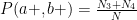
Now let us ask, what is the probability that in an arbitrary chosen pair the spin projection of the first particle on a axis is measured “up”(+), and spin projection of the second particle on b axis is measured “up”(+). From the table, these are pairs from the 3rd and 4th groups, so
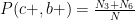
Similarly, we could find


and

Now

We derived one of the Bell inequalities

which should always be satisfied if Einstein was right.
5. Violation of Bell inequalities
It is easy to show that Bell inequalities can be violated in QM. Let a,b and c axes are lying in the same plane and c axis is lying between a and b axes, in the middle. From QM, the probability that projection of spin of the first particle on axis 

where 

The above inequality is wrong if 
Disclaimer: The derivation of Bell inequalities is taken from Barton Zwiebach’s course of QM MIT 8.05.
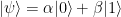
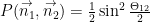
 and
and  are (up to a global phase) the quantum information stored in the qubit; instead of saying “qubit has state
  “, we can say “qubit store information
  of a pure state
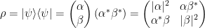
 and
and  are real,
  ,
,  , and
, and 

 or
or  , it just happened that we don’t know it exactly and model our incomplete knowledge by probabilities

 of being in state
 , where
  stands for xor operation.
 possible strategies. Since the probability of
  is 75%, it can be easily seen that there exists 75%-winning strategy – Alice and Bob simply ignore the questions and answer identically – either by bit 0 both or by bit 1 both; it seems natural that this is the best strategy, and it is indeed so, as can be formally shown by checking all 16 possible strategies.
 :
:

 on receiving the question 0, and
  on receiving the question 1; Bob uses
  on receiving the question 0, and
  on receiving the question 1.
 , Alice and Bob win if they answer identically
  or
or  . The correspondent probability of winning (given

 we get

 we get

 and
and  are similar to


 Alice and Bob win if they answer differently, so:


 , then

 (fig. 1). Quantum Mechanics (QM) states that if we measure the spin along z direction we get
  with probability
  and
and  with probability
  . There is no way to tell which result will be obtained; the uncertainty of measurement of non-commuting observables is a fundamental law of nature.
 (with probability
  (with probability
  direction the original state


 particle does not affect the
  particle in any way, and if we measure spin of the particle
 and
and  (fig.2). QM predicts that the probability of obtaining
  for the particle
  for the particle
  ; the other possibilities are
  ,
,  ,
,  , all add up to 1.
 of pairs having the particle
  and the particle
 of pairs having the particle
  and the particle
 for the particle
  for the particle
  as one should expect; if we measure spin of the particle


 and
and  and measure spin of the particle
  for spin of the particle
  . We have from the table above:


 ,
,
 (fig.3), then the inequality becomes

