Quantum Information and Quantum Noise

Posted on September 1, 2018 by Serg

The term quantum information is really a synonym of the term quantum state, only viewed at a different angle. If a qubit has state

$|\psi\rangle =\alpha|0\rangle + \beta|1\rangle$

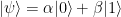
then the complex numbers $\alpha$ and $\beta$ are (up to a global phase) the quantum information stored in the qubit; instead of saying “qubit has state $|\psi\rangle$ “, we can say “qubit store information $|\psi\rangle$ ”

If we have a single qubit, we can’t pull down quantum information from the qubit into our classical world. We need many qubits storing identical information to measure $\alpha$ and $\beta$ with some precision; the more precision we want, the more qubits we need. We can’t also obtain $\alpha$ and $\beta$ by measuring in a single basis only, we need to measure in two different bases at least.

Pure states

$|\psi\rangle =\alpha|0\rangle + \beta|1\rangle$

are not the most general qubit’s states. The most general states are called mixed states and are described by density matrices. Density matrix $\rho$ of a pure state $|\psi\rangle$ is

$\rho =|\psi\rangle\langle\psi|=\begin{pmatrix}\alpha \\ \beta\end{pmatrix}(\alpha^* \beta^*)=\begin{pmatrix} |\alpha|^2 & \alpha\beta^* \\ \alpha^*\beta &|\beta|^2 \end{pmatrix}$

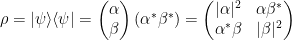
A valid density matrix must be Hermitian, positive semidefinite and have trace 1; vice versa, any Hermitian and positive semidefinite matrix with trace 1 is a valid density matrix.

An example of a density matrix of a non-pure state:

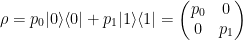
$\rho =p_0|0\rangle\langle 0|+p_1|1\rangle\langle 1|=\begin{pmatrix} p_0 & 0 \\ 0 &p_1 \end{pmatrix}$

where $p_0$ and $p_1$ are real, $p_0\geqslant 0$ , $p_1\geqslant 0$ , and $p_0 + p_1 = 1$

Non-pure states are also called noisy states. In the classical data processing noise is always bad and we should always get rid of the noise to obtain clean data. As we will see soon, the quantum noise is more interesting.

What does it mean that a qubit has mixed state

$\rho =\begin{pmatrix} p_0 & 0 \\ 0 &p_1 \end{pmatrix}$

Does it mean that a qubit really has a pure state $|0\rangle$ or $|1\rangle$ , it just happened that we don’t know it exactly and model our incomplete knowledge by probabilities $p_0$ and $p_1$ ?

Well, this is subtle. It is possible that a qubit has a pure state that we don’t know exactly, but it is also possible that a qubit has no pure state.

What is important to understand, the above said is not some philosophy. The difference between the two cases has mathematical consequences in quantum mechanics, and in the end of the day the difference can be (statistically) measured.

Let us consider two-qubit EPR state

$|\psi_{1}\rangle =\frac{1}{\sqrt{2}}(|00\rangle + |11\rangle)$

The density matrix of the state is

$\rho_{1} =\frac{1}{2}(|00\rangle + |11\rangle)(\langle 00| + \langle 11|)=\frac{1}{2}\begin{pmatrix} 1 & 0 & 0 & 1 \\ 0 & 0 & 0 & 0 \\ 0 & 0 & 0 & 0 \\ 1 & 0 & 0 & 1 \end{pmatrix}$

Each qubit in the pair the has probability $1/2$ of being in state $|0\rangle$ or state $|1\rangle$ .

We can construct mixed state with the same property:

$\rho_{2} =\frac{1}{2}(|00\rangle\langle 00| + |11\rangle\langle 11|)=\frac{1}{2}\begin{pmatrix} 1 & 0 & 0 & 0 \\ 0 & 0 & 0 & 0 \\ 0 & 0 & 0 & 0 \\ 0 & 0 & 0 & 1 \end{pmatrix}$

In both cases the individual qubits have identical noisy states (only the two-qubit states are different). It looks like the EPR state and the second state are statistically identical, but John Bell using clever argument has shown that they are not: EPR state violates so-called Bell’s inequalities while the second state does not.

It is funny that the Bell’s discovery happened about 30 years after the related questions were raised in the famous EPR paper by Einstein himself, and all prominent physicists of the time were aware of the EPR paper; the discovery has waited 30 years for John Bell.

It is common knowledge today that the density matrix formalism mathematically captures physical difference of the states: two states with the same density matrix are physically indistinguishable, and two states with different density matrices are physically distinguishable; it seems like nobody understood this before the Bell’s discovery.

Another term to discuss quantum noise is coherence (the term coherence may have different meanings in physics, be aware). If an initially pure qubit’s state evolves into a noisy state, we say that the qubit has lost coherence. But there are different ways to loose coherence. The coherence of an individual qubit in a multiqubit system may leak into other qubits of the system so that the whole multiqubit system preserves coherence. This is controllable and reversible loss of coherence. If the multiqubit system is quantum computer, this process is an important part of quantum computation. In the quantum algorithms the individual qubits loose coherence at intermediate step and restore coherence (with high probability at least) in the end, before the final measurement.

The main problem with building quantum computers is that coherence uncontrollably leaks into environment, and the whole multiqubit system looses coherence; since we can’t control environment on the quantum level, the loss of coherence is irreversible. This process introduces really bad kind of quantum noise which destroys quantum computation.

CHSH game in detail

Posted on October 26, 2016 by Serg

CHSH (John Clauser, Michael Horne, Abner Shimony, and Richard Holt) game is another view on the Bell’s inequalities, showing that under the hood our world is not classical. The game is played by Alice and Bob, and proceeds as follows:

a referee generates two independent uniformly chosen random bits (x and y, also called “questions”) and sends x bit to Alice and y bit to Bob
After receiving the questions, Alice and Bob send their answers back to the referee; an answer is one bit too (a for Alice and b for Bob)
Alice and Bob win if $x \cdot y = a \oplus b$ , where $\oplus$ stands for xor operation.

The game is cooperative – Alice and Bob do not play against each other, their goal is to get the highest winning probability together. Before the game starts, Alice and Bob can communicate and decide on the strategy they will use; after the game started, Alice and Bob are not allowed to communicate anymore; Alice doesn’t know what question the referee sent to Bob, and Bob doesn’t know what question the referee sent to Alice.

In the classical world, Alice and Bob have 16 possible deterministic strategies – both Alice and Bob have two possible answers for each of two possible questions, combining them we get $2^2 \cdot 2^2 = 16$ possible strategies. Since the probability of $x \cdot y = 0$ is 75%, it can be easily seen that there exists 75%-winning strategy – Alice and Bob simply ignore the questions and answer identically – either by bit 0 both or by bit 1 both; it seems natural that this is the best strategy, and it is indeed so, as can be formally shown by checking all 16 possible strategies.

In the quantum world, Alice and Bob have additional degree of freedom – before the game starts, they share an entangled bipartite state, for example two-qubit EPR state:

$|\Psi_{AB}\rangle = \frac{1}{\sqrt{2}}(|0\rangle_A\otimes|0\rangle_B + |1\rangle_A\otimes|1\rangle_B)$

Now, Alice and Bob choose the measurement bases according to the questions they receive from the referee, and answer by measuring their qubits in the chosen bases.

Let us denote the basis vectors as $\nu_i(\theta)$ :

Alice uses $\theta_{A0}$ on receiving the question 0, and $\theta_{A1}$ on receiving the question 1; Bob uses $\theta_{B0}$ on receiving the question 0, and $\theta_{B1}$ on receiving the question 1.

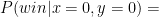
If the referee sends questions $x = 0, y = 0$ , Alice and Bob win if they answer identically $a = 0, b = 0$ or $a = 1, b = 1$ . The correspondent probability of winning (given $x = 0, y = 0$ ) is:

$P(win|x=0,y=0) =$
$|\langle_A\nu_0(\theta_{A0})|\otimes\langle_B\nu_0(\theta_{B0})|\Psi_{AB}\rangle|^2 + |\langle_A\nu_1(\theta_{A0})|\otimes\langle_B\nu_1(\theta_{B0})|\Psi_{AB}\rangle|^2$

Substituting $|\nu_i(\theta)\rangle$ we get
$P(win|x=0,y=0) =$
$|(\cos\theta_{A0} \langle_A 0| + \sin\theta_{A0} \langle_A 1|) \otimes (\cos\theta_{B0} \langle_B 0| + \sin\theta_{B0} \langle_B 1|)|\Psi_{AB}\rangle|^2 +$
$|(\sin\theta_{A0} \langle_A 0| - \cos\theta_{A0} \langle_A 1|) \otimes (\sin\theta_{B0} \langle_B 0| - \cos\theta_{B0} \langle_B 1|)|\Psi_{AB}\rangle|^2$

Substituting $|\Psi_{AB}\rangle$ we get
$P(win|x=0,y=0) =$
$\frac{1}{2}|\cos\theta_{A0} \cos\theta_{B0} + \sin\theta_{A0} \sin\theta_{B0}|^2 + \frac{1}{2}|\sin\theta_{A0} \sin\theta_{B0} + \cos\theta_{A0} \cos\theta_{B0}|^2$

Finally,
$P(win|x=0,y=0) = \cos^2 (\theta_{A0} - \theta_{B0})$

The cases $x = 0, y = 1$ and $x = 1, y = 0$ are similar to $x = 0, y = 0$ : Alice and Bob win if they answer identically:

$P(win|x=0,y=1) =$
$|\langle_A\nu_0(\theta_{A0})|\otimes\langle_B\nu_0(\theta_{B1})|\Psi_{AB}\rangle|^2 + |\langle_A\nu_1(\theta_{A0})|\otimes\langle_B\nu_1(\theta_{B1})|\Psi_{AB}\rangle|^2 =$
$|(\cos\theta_{A0} \langle_A 0| + \sin\theta_{A0} \langle_A 1|) \otimes (\cos\theta_{B1} \langle_B 0| + \sin\theta_{B1} \langle_B 1|)|\Psi_{AB}\rangle|^2 +$
$|(\sin\theta_{A0} \langle_A 0| - \cos\theta_{A0} \langle_A 1|) \otimes (\sin\theta_{B1} \langle_B 0| - \cos\theta_{B1} \langle_B 1|)|\Psi_{AB}\rangle|^2$

$P(win|x=0,y=1) = \cos^2 (\theta_{A0} - \theta_{B1})$

$P(win|x=1,y=0) =$
$|\langle_A\nu_0(\theta_{A1})|\otimes\langle_B\nu_0(\theta_{B0})|\Psi_{AB}\rangle|^2 + |\langle_A\nu_1(\theta_{A1})|\otimes\langle_B\nu_1(\theta_{B0})|\Psi_{AB}\rangle|^2=$
$|(\cos\theta_{A1} \langle_A 0| + \sin\theta_{A1} \langle_A 1|) \otimes (\cos\theta_{B0} \langle_B 0| + \sin\theta_{B0} \langle_B 1|)|\Psi_{AB}\rangle|^2 +$
$|(\sin\theta_{A1} \langle_A 0| - \cos\theta_{A1} \langle_A 1|) \otimes (\sin\theta_{B0} \langle_B 0| - \cos\theta_{B0} \langle_B 1|)|\Psi_{AB}\rangle|^2$

$P(win|x=1,y=0) =\cos^2 (\theta_{A1} - \theta_{B0})$

In the last case $x = 1, y = 1$ Alice and Bob win if they answer differently, so:

$P(win|x=1,y=1) =$
$|\langle_A\nu_0(\theta_{A1})|\otimes\langle_B\nu_1(\theta_{B1})|\Psi_{AB}\rangle|^2 + |\langle_A\nu_1(\theta_{A1})|\otimes\langle_B\nu_0(\theta_{B1})|\Psi_{AB}\rangle|^2=$

$|(\cos\theta_{A1} \langle_A 0| + \sin\theta_{A1} \langle_A 1|) \otimes (\sin\theta_{B1} \langle_B 0| - \cos\theta_{B1} \langle_B 1|)|\Psi_{AB}\rangle|^2 +$
$|(\sin\theta_{A1} \langle_A 0| - \cos\theta_{A1} \langle_A 1|) \otimes (\cos\theta_{B1} \langle_B 0| + \sin\theta_{B1} \langle_B 1|)|\Psi_{AB}\rangle|^2=$

$\frac{1}{2}|\cos\theta_{A1} \sin\theta_{B1} - \sin\theta_{A1} \cos\theta_{B1}|^2 + \frac{1}{2}|\sin\theta_{A1} \cos\theta_{B1} - \cos\theta_{A1} \sin\theta_{B1}|^2$

$P(win|x=1,y=1) = \sin^2 (\theta_{A1} - \theta_{B1})$

Putting it all together:

$P(win) = \frac{1}{4}(P(win|x=0,y=0) + P(win|x=0,y=1)+ P(win|x=1,y=0)+ P(win|x=1,y=1)) =$
$\frac{1}{4}(\cos^2 (\theta_{A0} - \theta_{B0})+\cos^2 (\theta_{A0} - \theta_{B1})+\cos^2 (\theta_{A1} - \theta_{B0})+\sin^2 (\theta_{A1} - \theta_{B1}))$

if Alice and Bob choose $\{\theta_{A0}=0, \theta_{A1}=\frac{\pi}{4}, \theta_{B0}=\frac{\pi}{8}, \theta_{B1}=-\frac{\pi}{8}\}$ , then

$P(win) = \frac{3}{4} \cos^2 \frac{\pi}{8} + \frac{1}{4} \sin^2 \frac{3\pi}{8}= \cos^2 \frac{\pi}{8} = \frac{1+cos \frac{\pi}{4}}{2}= \frac{1}{2} + \frac{1}{2\sqrt{2}}\approx 0.85355$

and we obtain the winning probability above 85%, which is significantly better than classical 75%.

Notes on EPR Paradox, Entanglement and Bell’s Inequality

Posted on June 22, 2015 by Serg

1. Elements of reality (aka hidden variables) vs uncertainty.

Suppose we have a spin-1/2 particle (ex electron) in the state $|n+\rangle$ (fig. 1). Quantum Mechanics (QM) states that if we measure the spin along z direction we get $|z+\rangle$ with probability $cos^2(\theta/2)$ and $|z-\rangle$ with probability $sin^2(\theta/2)$ . There is no way to tell which result will be obtained; the uncertainty of measurement of non-commuting observables is a fundamental law of nature.

Einstein, Podolsky and Rosen (EPR) say – no, there is nothing fundamental here. The particle has elements of reality which determine the measurement result in a unique deterministic way; the particle is either of type $(z+,n+)$ (with probability $cos^2(\theta/2)$ ), or of type $(z-,n+)$ (with probability $sin^2(\theta/2)$ ), but not of both types at the same time. Statistically the results of spin measurements exactly reproduce the QM predictions.

2. Entanglement.

QM rules out the “elements of reality” because generally they cannot be measured simultaneously; if we have a particle in state $|n+\rangle$ and measure spin along $z$ direction the original state $|n+\rangle$ “collapses” either to $|z+\rangle$ or to $|z-\rangle$ and does not “exist” anymore.

EPR say – no, this does not seem to be true because we can measure a particle’s spin without acting on the particle. Suppose we have the singlet state of two spin-1/2 particles A and B:

$\psi = \frac{1}{\sqrt{2}}(|+\rangle_A\otimes|-\rangle_B - |-\rangle_A\otimes|+\rangle_B)$

this state is fully invariant under rotations, so it can be written as

$\psi = \frac{1}{\sqrt{2}}(|z+\rangle_A\otimes|z-\rangle_B - |z-\rangle_A\otimes|z+\rangle_B)$

$\psi = \frac{1}{\sqrt{2}}(|n+\rangle_A\otimes|n-\rangle_B - |n-\rangle_A\otimes|n+\rangle_B)$

We can create an experimental setup such that a spin measurement on the $A$ particle does not affect the $B$ particle in any way, and if we measure spin of the particle $A$ along some direction then spin of the particle $B$ is always opposite, so in the end we measure spin of the particle $B$ without disturbing it.

N.B. Prior to the measurement the particles $A$ and $B$ had no (pure) states of their own, only the common 2-particle singlet state. The measurement does not really “collapse” a state of the particle $B$ because it had no (pure) state before the measurement but instead “create” a (pure) state of the particle $B$ .

3. EPR paradox.

The challenge of EPR is to reproduce all statistical QM predictions using the classical concept of “elements of reality”. As an example let us consider the same singlet state and measure spins of the particles $A$ and $B$ along two different directions $z_1$ and $z_2$ (fig.2). QM predicts that the probability of obtaining $|z_1+\rangle$ for the particle $A$ and $|z_2+\rangle$ for the particle $B$ is equal to $P(++)=\frac{1}{2}sin^2(\theta/2)$ ; the other possibilities are $P(+-)=\frac{1}{2}cos^2(\theta/2)$ , $P(-+)=\frac{1}{2}cos^2(\theta/2)$ , $P(--)=\frac{1}{2}sin^2(\theta/2)$ , all add up to 1.

EPR say: in this experiment we have following statistical mixture of pairs of particles:

a fraction $\frac{1}{2}cos^2(\theta/2)$ of pairs having the particle $A$ of type $(z_1+,z_2+)$ and the particle $B$ of type $(z_1-,z_2-)$
a fraction $\frac{1}{2}sin^2(\theta/2)$ of pairs having the particle $A$ of type $(z_1+,z_2-)$ and the particle $B$ of type $(z_1-,z_2+)$
a fraction $\frac{1}{2}sin^2(\theta/2)$ of pairs having the particle $A$ of type $(z_1-,z_2+)$ and the particle $B$ of type $(z_1+,z_2-)$
a fraction $\frac{1}{2}cos^2(\theta/2)$ of pairs having the particle $A$ of type $(z_1-,z_2-)$ and the particle $B$ of type $(z_1+,z_2+)$

It can be seen that the mixture reproduces the QM predictions whether we measure the spins along the same direction or along different directions. For example, if we measure the spins of both particles along $z_1$ then the probability of obtaining $+$ for the particle $A$ and $-$ for the particle $B$ is equal to the sum of fractions (1) and (2), giving $\frac{1}{2}cos^2(\theta/2) + \frac{1}{2}sin^2(\theta/2)=\frac{1}{2}$ as one should expect; if we measure spin of the particle $A$ along $z_1$ and spin of the particle $B$ along $z_2$ , then the probability of obtaining $+$ for the particle $A$ and $-$ for the particle $B$ is equal to the fraction (1), giving $\frac{1}{2}cos^2(\theta/2)$ , again consistent with QM prediction.

It turns out that it is not easy to propose an experiment disproving the EPR paradox.

4. Bell’s inequality.

Let us take the same 2-particle singlet state, but now measure spins along 3 directions (fig.3). Using the EPR’s “elements of reality” framework, the statistical mixture consists of 8 fractions of pairs of the particles $A$ and $B$ :

fraction	particle $A$	particle $B$
$P_1$	$(z_1+,z_2+,z_3+)$	$(z_1-,z_2-,z_3-)$
$P_2$	$(z_1+,z_2+,z_3-)$	$(z_1-,z_2-,z_3+)$
$P_3$	$(z_1+,z_2-,z_3+)$	$(z_1-,z_2+,z_3-)$
$P_4$	$(z_1+,z_2-,z_3-)$	$(z_1-,z_2+,z_3+)$
$P_5$	$(z_1-,z_2+,z_3+)$	$(z_1+,z_2-,z_3-)$
$P_6$	$(z_1-,z_2+,z_3-)$	$(z_1+,z_2-,z_3+)$
$P_7$	$(z_1-,z_2-,z_3+)$	$(z_1+,z_2+,z_3-)$
$P_8$	$(z_1-,z_2-,z_3-)$	$(z_1+,z_2+,z_3+)$

We choose 2 directions $z_i$ and $z_j$ and measure spin of the particle $A$ along $z_i$ and spin of the particle $B$ along $z_j$ .
Let us denote the probability of obtaining $(+)$ for spin of the particle $A$ and $(+)$ for spin of the particle $B$ as $P_{ij}$ . We have from the table above:

$P_{12}=P_3+P_4$
$P_{13}=P_2+P_4$
$P_{32}=P_3+P_7$

Using little algebra

$P_{13}+P_{32}=P_2+P_4+P_3+P_7=P_{12}+P_2+P_7 \ge P_{12}$ ,

or finally

$P_{12} \le P_{13} + P_{32}$

But this inequality is easily violated in QM. Let us consider a planar configuration of the axis $z_i$ and choose $\theta_{13}=\theta_{32}=\theta$ (fig.3), then the inequality becomes

$\frac{1}{2}sin^2(\theta) \le sin^2(\theta/2)$

which is wrong for any $\theta < \pi/2$

The result can be formulated as the Bell’s theorem:

No physical theory of local hidden variables can ever reproduce all of the predictions of quantum mechanics.

The Programming Works

Delphi programming and more

Tag Archives: Quantum Mechanics

Quantum Information and Quantum Noise

CHSH game in detail

Notes on EPR Paradox, Entanglement and Bell’s Inequality